
A distillation column begins to drift from its target purity during a busy production shift. Steam pressure has changed, feed composition is moving, and an operator sees several trend lines bend away from their usual paths. The immediate question is simple: which valve should move, by how much, and when?
In a small system, an experienced operator may recognize the pattern and intervene quickly. In a modern plant, however, hundreds or thousands of measurements change together. A corrective action that improves one variable can upset energy use, throughput, emissions, equipment limits, or a downstream unit.
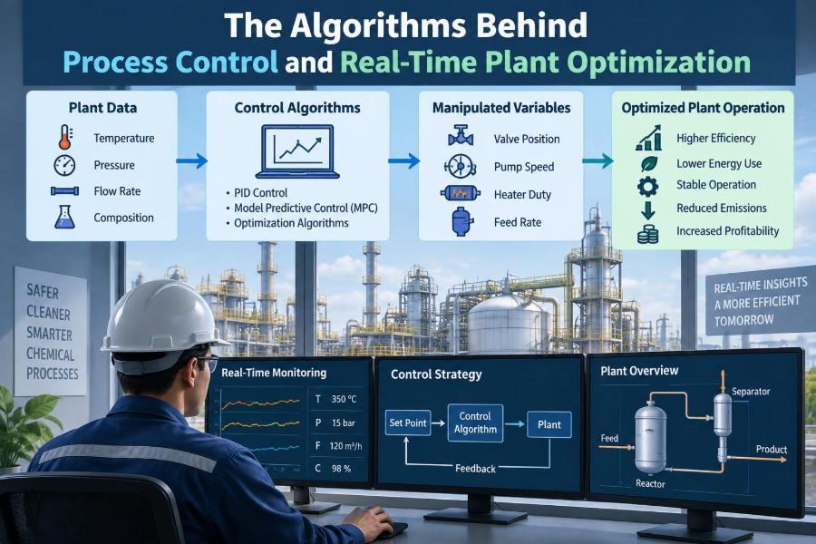
That is why process control is not just about holding a temperature or pressure steady. It is a continuous decision problem: measure the process, infer what is happening, predict what may happen next, and choose an action within safe operating limits.
The algorithms behind those decisions range from the familiar proportional-integral-derivative controller to model predictive control, state estimation, optimization, and carefully governed machine-learning tools. Understanding their roles helps engineers use automation intelligently rather than treating it as a black box.
🏭 Process Control Is Coordinated Decision-Making
Process control uses measurements and manipulated inputs to keep a process near desired operating conditions. A controlled variable might be reactor temperature, tank level, product composition, or column pressure. A manipulated variable is an input the system can adjust, such as a valve position, heater duty, compressor speed, or reflux flow.
Most real plants are interconnected. Raising reflux in a distillation column may improve overhead purity, but it also changes condenser duty, reboiler load, hydraulic behavior, and energy consumption. Control algorithms exist to manage these interactions repeatedly and reliably.
📡 Measurements Are the Algorithm’s View of Reality
No controller sees a process directly. It sees sensor signals: temperatures, pressures, flows, levels, analyzer readings, motor currents, vibration data, and laboratory results. Those signals may be delayed, noisy, biased, intermittent, or located far from the variable that truly matters.
This creates a practical distinction between what is measured and what is known. A temperature transmitter may report a precise number, but a fouled thermowell, poor installation, or calibration drift can still make that number misleading.
Good optimization starts with a basic rule: poor measurements cannot be repaired merely by sophisticated mathematics.
🔁 Feedback Control Corrects Deviations
Feedback control compares a measurement with a target called the setpoint. The difference is the error. If a vessel level rises above setpoint, the controller may open an outlet valve; if it falls below setpoint, the valve may close.
Feedback is powerful because it responds to disturbances without needing to know their exact cause. A change in feed rate, ambient temperature, or upstream pressure can all be corrected if their effects appear in the measured variable.
Its limitation is timing: feedback acts only after a deviation is detectable. For slow analyzers or long process delays, waiting for the final product measurement may be too late for a sharp correction.
🎚️ PID Control Remains the Workhorse
The proportional-integral-derivative, or PID, controller is widely used because it is understandable, adaptable, and effective for many single-loop tasks. Its three terms respond to present error, accumulated past error, and the rate at which error is changing.
| PID term | What it responds to | Practical role |
|---|---|---|
| Proportional | Current error | Provides an immediate corrective push |
| Integral | Persistent error over time | Removes steady offset from the setpoint |
| Derivative | Rate of error change | Can anticipate rapid movement, but is sensitive to noise |
A temperature loop on a jacketed reactor may use PID to regulate steam flow. If the reactor cools, proportional action increases steam promptly; integral action continues adjusting until the target is recovered.
PID is not obsolete because advanced control exists. It is the dependable regulatory layer beneath much of advanced automation.
🧭 Setpoints Are Operating Decisions, Not Just Numbers
A PID loop answers, “How do I reach this setpoint?” It generally does not answer, “What should the setpoint be right now?” The second question belongs to supervisory control and optimization.
For example, a flow controller may hold reflux flow at its target very well. An optimizer may periodically calculate a better reflux target based on feed quality, utility limits, product specifications, and expected economic trade-offs.
This hierarchy prevents confusion. Regulatory control stabilizes the process; higher-level algorithms select targets that make operational sense.
🪜 Cascade Control Handles Fast Inner Dynamics
Cascade control uses two nested loops. The outer loop controls the main variable and sends a setpoint to a faster inner loop. A reactor temperature controller, for instance, can set the target for a steam-flow controller rather than positioning a steam valve directly.
The inner flow loop reacts quickly to steam pressure changes or valve nonlinearities. The outer temperature loop then sees a more predictable heating response.
Cascade works only when the inner loop is genuinely faster and properly tuned. Adding loops without understanding the process can create unstable or confusing behavior.
🔮 Feedforward Acts Before the Error Arrives
Feedforward control uses a measurable disturbance to calculate a corrective action before the controlled variable moves. If a furnace feed flow increases and that flow is measured, fuel can be adjusted immediately instead of waiting for outlet temperature to fall.
It is often paired with feedback. Feedforward handles the known disturbance quickly, while feedback corrects model mismatch and unmeasured disturbances.
The trade-off is that feedforward needs a credible process relationship. A poorly maintained flowmeter or an oversimplified gain can make proactive correction worse than patient feedback.
🧱 Constraints Define the Safe Operating Envelope
Plants do not operate in an unlimited mathematical space. They have hard and soft constraints: maximum pressure, minimum pump flow, valve travel limits, compressor surge margins, allowable temperatures, emissions limits, and product-quality requirements.
A process may have an economically attractive target that is physically inaccessible at the moment. For example, increasing reactor throughput could exceed cooling capacity or push a downstream separator toward flooding.
Optimization must respect constraints before it pursues profit, energy reduction, or production rate. Safety instrumented functions and relief systems are separate protection layers, not optimization tools.
🧩 Multivariable Systems Create Interaction Problems
Many processes have multiple inputs affecting multiple outputs. In a distillation column, reflux and boilup both influence product compositions, while pressure shifts vapor-liquid equilibrium and condenser behavior.
If separate single-loop controllers are tuned without considering interaction, one loop may undo another’s work. The result can be oscillation, excessive valve motion, or slow quality recovery.
Engineers often begin with pairing analysis, process knowledge, and careful loop design. When interactions are strong, a multivariable strategy may be more appropriate.
📐 Process Models Turn Behavior into Equations
A process model is a representation of how inputs, states, disturbances, and outputs are related. It can be a first-principles model based on mass balances, energy balances, thermodynamics, and transport phenomena, or an empirical model estimated from operating data.
A heat exchanger model may relate inlet flows, temperatures, heat-transfer performance, and outlet temperature. A simple model does not need to capture every physical detail; it needs enough fidelity for the decision it will support.
Models are always approximations. Their value depends on the operating region, data quality, and whether important mechanisms have been omitted.
🧪 First-Principles and Data-Driven Models Serve Different Needs
First-principles models are attractive when physical relationships are understood and extrapolation beyond routine data is required. They can also make engineering assumptions visible, which aids review and troubleshooting.
Data-driven models learn input-output patterns from plant history or designed tests. They can be useful where physics is complex, measurements are abundant, and operation stays near the data used for training.
Neither approach automatically wins. Hybrid models often combine physical structure with data-based corrections, offering a useful balance between interpretability and practical accuracy.
⏱️ Dynamics and Dead Time Shape Every Control Problem
Processes do not respond instantly. A jacket temperature may react within minutes, a large tank level may take much longer, and a composition analyzer may add sampling and measurement delay. Dead time is the delay before an input change has a visible effect.
Long delay makes aggressive feedback risky because the controller can keep correcting an error that has already been addressed but has not yet appeared in the measurement. The familiar result is overshoot and cycling.
Dynamic models capture this time-dependent behavior. They are essential for tuning, prediction, and safe online optimization.
🧠 State Estimation Fills in What Sensors Cannot Measure
A process state is an internal condition that affects future behavior, such as vessel inventory distribution, catalyst activity, unmeasured composition, or thermal storage. Not all states are measured continuously or economically.
A state estimator combines a model with noisy measurements to estimate these hidden quantities. Kalman-filter variants are common examples in systems with uncertainty and frequent measurements.
An estimator is not a license to ignore instruments. It supplies an informed estimate, and its reliability must be monitored against measurements and process knowledge.
🧹 Signal Filtering Must Remove Noise Without Hiding Change
Raw sensor signals often contain noise. Filtering can prevent controllers from chasing random fluctuations and can make trends easier to interpret. But excessive filtering adds delay, exactly what many loops cannot tolerate.
The right question is not “How smooth does the trend look?” It is “Does this treatment preserve the information needed for a timely and stable decision?”
For critical loops, engineers should inspect both the unfiltered signal and the filtered signal during disturbances. A visually tidy trend can conceal a controller that reacts too late.
🧮 Model Predictive Control Looks Ahead
Model predictive control (MPC) uses a dynamic model to forecast how the process will evolve over a future time horizon. At each control interval, it evaluates possible moves and selects actions that best satisfy objectives while honoring constraints.
Only the first part of the calculated move is applied. At the next interval, new measurements are received, the prediction is updated, and the calculation is repeated. This is often called a receding-horizon approach.
MPC is particularly useful for processes with interactions, delays, slow analyzers, and operating constraints—common conditions in furnaces, fractionation systems, grinding circuits, and utility networks.
⚖️ The MPC Objective Balances Competing Priorities
An MPC calculation typically penalizes deviation from important targets, unnecessary movement of manipulated variables, and violation of constraints. It does not seek a single perfect response; it makes trade-offs explicitly.
Consider a hypothetical column approaching a pressure limit while overhead purity starts to fall. MPC may choose moderated changes in reflux and boilup, rather than forcing purity recovery through a move that violates pressure or overwhelms utilities.
The chosen weights matter. If production is weighted too heavily, the controller may operate uncomfortably close to limits. If move suppression is too strong, it may respond sluggishly to real disturbances.
💰 Real-Time Optimization Chooses the Best Operating Targets
Real-time optimization (RTO) operates above regulatory control and often above MPC. Its purpose is to determine economically favorable targets using current estimates of process conditions, constraints, prices or costs, equipment performance, and product requirements.
A typical RTO problem might minimize fuel use while meeting product quality and throughput commitments. Another might distribute feed among parallel units while respecting capacity and maintenance limitations.
RTO does not replace operators or safety systems. It supplies recommended or automatically implemented targets to control layers that execute them safely.
📈 Economics Must Be Expressed as a Real Objective
“Maximize profit” is too vague for an algorithm. The objective must be translated into terms the system can evaluate: energy consumption, yield loss, utility cost, product value, off-spec risk, or equipment wear.
Some costs are difficult to quantify. Frequent valve movement may shorten equipment life, and operating near a quality boundary may increase the chance of costly off-spec material. These effects may require conservative constraints or operational rules rather than a simplistic monetary estimate.
Transparent objectives are easier for engineers and operators to challenge, improve, and trust.
🧫 Quality Control Often Depends on Inference
Key quality variables may be measured only by laboratory testing or analyzers with long cycle times. Waiting for a delayed result can allow a large amount of material to move through the process before correction begins.
A soft sensor, also called an inferential measurement, estimates quality from faster signals such as temperatures, pressures, flows, spectra, and operating conditions. It can provide a frequent quality estimate between laboratory results.
Soft sensors must be validated and recalibrated. Changes in feedstock, catalyst condition, sensor health, or operating regime can gradually break the relationship on which the estimate depends.
🗂️ Historian Data Is Valuable but Not Automatically Ready
Plant historians store a rich record of operations, but historical data includes bad timestamps, maintenance periods, manual interventions, sensor failures, clipped values, and periods when the process was deliberately unstable.
Before using data for model identification or machine learning, engineers need contextual cleaning. A flat-lined transmitter is not a stable process; it may be a failed instrument. A sudden step may be a grade change rather than a normal disturbance.
Data preparation requires process knowledge, not just software. The people who understand shutdowns, operating modes, and instrumentation often determine whether an analytics project succeeds.
🤖 Machine Learning Has a Focused Role
Machine learning can detect patterns in high-dimensional data, estimate difficult-to-measure variables, classify operating modes, and flag unusual behavior. It can be useful where mechanistic models are costly or incomplete.
Its limits are equally relevant. A model trained on normal operation may be unreliable during start-up, shutdown, major feed changes, or rare abnormal events. Correlation can also mistake a coincidental operating pattern for a causal relationship.
For control actions with material safety, environmental, or production consequences, machine-learning outputs need clear bounds, validation, monitoring, and a defined human or automated fallback path.
🛎️ Alarm Management Prevents Attention Overload
Alarms tell people when intervention is required; they are not a substitute for control design. An alarm flood can overwhelm an operator just when situational awareness is most needed.
Effective alarm design distinguishes among notifications, operating alerts, and conditions requiring prompt action. Each alarm should have a rational purpose, a meaningful priority, and an expected response.
If a controller repeatedly drives a variable into alarm, silencing the alarm treats the symptom. The underlying problem may be poor tuning, a damaged valve, an infeasible target, or an unrecognized process constraint.
🛡️ Safety Layers Must Remain Independent
Basic process control systems regulate normal operation. Alarms support operator response. Safety instrumented systems and mechanical protections address hazardous scenarios when normal control is insufficient.
An optimizer should never be treated as a protective layer simply because it usually respects limits. Models can be wrong, measurements can fail, communications can be interrupted, and optimization objectives can be configured incorrectly.
Clear separation of purpose makes automation safer: optimization seeks better operation; independent protection manages credible hazards.
👷 Operators Need Visibility and Authority
Automation works best when operators can see what it is doing and why. Useful interfaces show active constraints, controller modes, key predictions, target changes, manipulated-variable movement, and reasons for any recommendation.
Operators also need practical ways to place applications in advisory mode, hold targets, transfer control safely, and report suspicious behavior. An unexplained algorithm is more likely to be bypassed, especially during a difficult shift.
Involving operators during design reveals realities that trend data may miss: sticking valves, sampling habits, equipment quirks, grade-transition practices, and operational constraints not written in a model.
🔧 Tuning Is an Ongoing Maintenance Task
Control tuning is not a one-time commissioning event. Valve friction changes, heat-transfer surfaces foul, feedstocks vary, equipment is modified, and production objectives evolve. A loop that was stable last year may now oscillate or respond too slowly.
Useful performance indicators include variability around target, time spent near constraints, valve travel, oscillation frequency, manual-mode usage, and the gap between inferred and laboratory quality.
Performance monitoring should lead to diagnosis, not automatic blame. A poorly performing loop may be revealing a mechanical issue or a process limitation rather than a bad controller setting.
🧰 Common Failure Modes Are Usually Practical
Advanced projects rarely fail because the optimization mathematics is impossible. More often, the difficulty lies in implementation details that were underestimated.
- Bad actuator behavior: deadband, stiction, incorrect valve sizing, or unreliable position feedback.
- Unclear ownership: no team is responsible for model upkeep, target approval, or performance review.
- Changing operating modes: one model is applied across grades, rates, or equipment configurations where it no longer fits.
- Hidden constraints: experienced operators know a limit that has never been encoded in the application.
- Weak change management: plant modifications occur without checking their impact on models and control logic.
Addressing these fundamentals often produces more value than adding another layer of algorithmic complexity.
🧭 A Sensible Implementation Sequence
A staged approach reduces risk and builds confidence. Begin by identifying the business or operational problem precisely: excessive energy use, poor quality consistency, limited throughput, unstable operation, or frequent constraint violations.
- Verify instrumentation, final control elements, and basic regulatory loops.
- Define operating objectives, constraints, modes, and safe fallback behavior.
- Collect representative data and develop models appropriate to the decision.
- Test using simulation, historical replay, or a controlled commissioning plan.
- Introduce advisory recommendations before increasing automation where appropriate.
- Monitor results, maintain models, and manage changes throughout the lifecycle.
This sequence is deliberately unglamorous. It reflects the fact that dependable optimization rests on dependable operations.
🌐 Digital Twins Support Testing and Learning
A digital twin is a digital representation of a physical asset or process, ranging from a simple dynamic simulator to a connected model updated with plant data. It can help teams test control strategies, train operators, evaluate disturbances, and compare proposed operating policies.
Its usefulness depends on its intended purpose. A high-fidelity simulation may be justified for operator training or major design decisions, while a simpler model may be sufficient for controller tuning studies.
A twin should not be assumed identical to the plant. Maintaining credibility requires periodic comparison with actual behavior and documented limits on where the model can be trusted.
🔐 Cybersecurity and Reliability Are Control Requirements
Connected optimization systems introduce interfaces among control networks, historians, analytics platforms, engineering workstations, and sometimes remote support tools. These interfaces need disciplined access control, network segmentation, backup practices, patch management, and incident response planning.
Availability matters too. If an optimizer becomes unavailable, the plant should continue in a stable, understood fallback mode. Regulatory control must not depend on a fragile analytics connection.
Cybersecurity and reliability are not separate IT concerns when software can influence physical equipment. They are part of responsible process engineering.
📚 Skills That Make Control Engineers Effective
Strong practitioners combine several disciplines. They understand mass and energy balances, dynamics, instrumentation, control theory, numerical methods, data quality, economics, safety philosophy, and plant operations.
Communication is equally valuable. A technically correct model that cannot be explained to operators, maintenance personnel, and management will struggle to survive commissioning and later plant changes.
For students, practical exercises with simulations, trend interpretation, PID tuning, and constrained optimization build useful intuition. For experienced engineers, time in the field remains one of the best ways to understand what algorithms must cope with.
🧩 The Core Principle: Better Decisions Within Better Boundaries
Process control and real-time optimization are often described as a ladder: sensors provide observations, regulatory loops stabilize the process, advanced controllers coordinate interacting variables, and optimizers choose better targets. The ladder works only when each layer is credible.
The goal is not maximum automation for its own sake. It is repeatable, understandable decision-making that improves performance while preserving operating discipline, equipment integrity, environmental compliance, and safety margins.
When a model, controller, or optimizer is uncertain, the correct response is not to hide the uncertainty. It is to recognize the limit, constrain the action, validate the assumptions, and retain safe fallback behavior.
The best plant algorithms do not replace engineering judgment; they make that judgment more consistent, timely, and usable at the scale of a real operating plant.
From a single PID loop to a constrained real-time optimizer, the same foundation applies: trustworthy data, sound process understanding, clear objectives, and respect for physical limits. Build those well, and automation becomes a practical partner in better chemical engineering decisions. 🧪⚙️📈