We want to turn up the radio because it’s noisy outside, and we want to hear what is broadcast. We therefore turn the volume knob toward ‘LOUD’. At its most basic, the volume control is a variable resistor, across which we pass a current from the battery, acting much like a kettle element. If we turn up the volume control then a larger current is allowed to flow, causing more energy to be produced by the resistor. As a listener, we hear a response because the sound from the speakers becomes louder. The speakers work harder. But we must be careful about the way we state these relationships. We do not ‘turn We consciously, carefully, vary the magnitude of the controlled variable and look at the response of the observed variable. up the volume’ (although in practice we might say these exact words and think in these terms). Rather, we vary the volume control and, as a response, our ears experience an increase in the decibels coming through the radio’s speakers. The listener controls the magnitude of the noise by deciding how far the volume-control knob needs to be turned. Only then will the volume change.
The process does not occur in reverse: we do not change the magnitude of the noise and see how it changes the position of the volume-control knob. While the magnitude of the noise and the position of the volume knob are both variables, they represent different types, with one depending on the other. The volume control is a controlled variable because the listener dictates its position. The amount of noise is the observed variable because it only changes in response to variations in the controlled variable, and not before.
Relationships and graphs
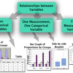
Physical chemists often depict relationships between variables by The x-axis (horizontal) is sometimes called the abscissa and the y-axis (vertical) is the ordinate. A simple way to remember which axis is which is to say, ‘an eXpanse of road goes horizontally along the x-axis’, and ‘a YoYo goes up and down the y-axis’. drawing graphs. The controlled variable is always drawn along the x-axis, and the observed variable is drawn up the y-axis. Figure 1.1 shows several graphs, each demonstrating a different kind of relationship. Graph (a) is straight line passing through the origin.
This graph says: when we vary the controlled variable x, the observed variable y changes in direct proportion. An obvious example in such a case is the colour intensity in a glass of blackcurrant cordial: the intensity increases in linear proportion to the concentration of the cordial, according to the Beer–Lambert law (see Chapter 9). Graph (a) in Figure 1.1 goes through the origin because there is no purple colour when there is no cordial (its concentration is zero). Graph (b) in Figure 1.1 also demonstrates the existence of a relationship between the variables x and y, although in this case not a linear relationship. In effect, the graph tells us that the observed variable y increases at a faster rate than does the controlled variable x. A simple example is the distance travelled by a ball as a function of time t as it accelerates while rolling down a hill. Although the graph is not straight, we still say there is a relationship, and still draw the controlled variable along the x-axis.

Graph (c) in Figure 1.1 is a straight-line graph, but is horizontal. In other words, whatever we do to the controlled variable x, the observed variable y will not change. In this case, the variable y is not a function of x because changing x will not change y. A simple example would be the position of a book on a shelf as a function of time. In the absence of other forces and variables, the book will not move just because it becomes evening.
Comments are closed