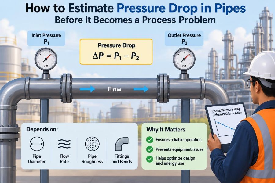

A pump is running, the flowmeter says production is below target, and someone proposes increasing pump speed. That response may work temporarily—but it can also hide the real issue: the system is losing more pressure than the original design allowed for.
Pressure drop is easy to overlook because pipes appear passive. Yet every metre of pipe, fitting, valve, strainer, elevation change, and process restriction consumes part of the pressure supplied by a pump or available from an upstream vessel.
For students, pressure-drop estimation turns fluid mechanics into a practical design tool. For operating engineers, it provides a disciplined way to ask why a line no longer delivers the required flow, why a control valve is nearly fully open, or why energy use has increased.
The goal is not to predict every pascal perfectly on the first pass. It is to make a defensible estimate, identify the dominant losses, and know when the result calls for better data or a more detailed hydraulic model.
🧭 Start with the pressure balance
A piping calculation begins with a pressure balance between two defined locations. For a horizontal line carrying a single liquid, the pump or upstream pressure must overcome frictional losses and any downstream pressure requirement.
In a more complete form, the energy balance includes pressure, velocity, elevation, pump head, turbine head, and losses. Written in head form, a common engineering expression is P₁/(ρg) + v₁²/(2g) + z₁ + Hpump = P₂/(ρg) + v₂²/(2g) + z₂ + hL.
The total loss term, hL, includes both pipe friction and local losses. Defining the endpoints clearly prevents a common error: calculating pipe friction accurately while forgetting the pressure that must still remain at the destination.
📉 What pressure drop actually means
Pressure drop is the reduction in static pressure between two points in a flowing system. In ordinary pipe flow, fluid near the wall is slowed by viscosity, while the faster core transfers momentum toward the wall. That irreversible process converts useful mechanical energy into heat.
Pressure drop is not always “bad.” A pressure-control valve intentionally creates it, and a restriction may be necessary for flow distribution or measurement. It becomes a process problem when the available pressure is insufficient for the required flow, equipment, or operating margin.
For incompressible liquids, engineers often express the same loss as pressure, head, or energy per unit mass. Choosing one basis and staying consistent is more valuable than choosing a fashionable unit system.
🧮 Separate major losses from minor losses
Major losses occur along the straight length of pipe. Despite the name, they are not always the largest contribution; “major” simply means distributed friction.
Minor losses occur at localized disturbances: elbows, tees, valves, reducers, entrances, exits, strainers, flowmeters, and other components. In a short, crowded skid, minor losses can exceed the loss in the straight pipe.
The total pressure drop is usually found by adding both contributions. A useful early question is therefore not “what is the pipe loss?” but “what is the complete flow path?”
📏 Define the system before choosing equations
Sketch the line from source to destination and mark every item that affects flow. Record pipe sizes, nominal lengths, elevations, material, fittings, valves, instruments, and known pressures or equipment duties.
Also define the operating case. A transfer line may see a normal flow, a maximum production flow, a low-flow recirculation case, and an occasional cleaning flow. One calculation cannot represent all of them if fluid properties or flow paths change.
- Where does the calculation start and end?
- What flow rate is required, not merely expected?
- Which valves are open, throttled, bypassed, or partially closed?
- What temperature and composition apply at that condition?
This simple inventory often exposes missing information before it becomes a spreadsheet problem.
🌊 Convert flow rate into velocity
Velocity links the process flow rate to friction. For a full circular pipe, calculate it from v = Q/A, where Q is volumetric flow rate and A = πD²/4 is the internal flow area.
Use the actual internal diameter, not just the nominal pipe size. Schedule, lining, corrosion allowance, and tube-versus-pipe designation can change the bore enough to matter, particularly in small lines.
Velocity rises sharply as diameter falls because area varies with diameter squared. If the same flow passes through a pipe with half the internal diameter, velocity becomes four times higher. That change is the beginning of a much larger friction penalty.
🔢 Calculate the Reynolds number
The Reynolds number indicates whether viscous effects or inertial effects dominate the flow pattern. For pipe flow, use Re = ρvD/μ, where ρ is density and μ is dynamic viscosity.
Low Reynolds number usually indicates laminar flow, where fluid moves in relatively orderly layers. Higher values usually indicate turbulent flow, with strong mixing and a friction factor that depends on wall roughness as well as Reynolds number.
The transition region is not a comfortable place for overconfidence. Its behavior can be sensitive to disturbances and geometry, so a calculation there deserves conservative assumptions and, when warranted, measured verification.
🧱 Use the Darcy–Weisbach equation
The Darcy–Weisbach equation is the general starting point for straight-pipe friction: ΔP = f(L/D)(ρv²/2). Here, f is the Darcy friction factor, L is pipe length, and D is internal diameter.
The equation works across a wide range of fluids and pipe materials when the friction factor is chosen appropriately. It is more broadly useful than empirical water-line shortcuts because it directly accommodates viscosity, density, diameter, velocity, and roughness.
Be careful with terminology. The Darcy friction factor is four times the Fanning friction factor. Mixing those definitions produces an error large enough to send a design in the wrong direction.
🌀 Choose the friction factor carefully
For fully developed laminar flow in a circular pipe, the Darcy friction factor is straightforward: f = 64/Re. Roughness has little influence in this regime because viscous resistance dominates.
For turbulent flow, the factor depends on Reynolds number and relative roughness, ε/D. Engineers may use the Moody chart, the Colebrook equation, or an explicit approximation such as Swamee–Jain. The method matters less than using it consistently and documenting the roughness assumption.
Commercial “smooth” pipe is not perfectly smooth, and aged pipe is not necessarily represented by new-pipe roughness. Deposits, corrosion, scaling, and liner degradation can increase resistance substantially over service life.
🧪 Treat fluid properties as operating data
Density and viscosity are not fixed labels attached to a fluid name. They vary with temperature, pressure, and composition; multiphase mixtures may not have a single meaningful viscosity for a simple calculation.
Temperature is especially influential for viscous liquids. A line that transfers easily at a warm operating temperature may develop excessive pressure drop during cold startup, winter operation, or an extended shutdown.
Use properties at the expected flowing condition, not a convenient value from a generic data sheet. When composition is uncertain, calculate a reasonable range rather than presenting one precise-looking but fragile answer.
📐 Account for internal diameter and pipe schedule
Nominal pipe size identifies a family of pipe dimensions, not one unique bore. A larger wall thickness reduces internal diameter, which raises velocity and normally increases pressure drop.
This matters most in small-diameter piping, where a modest bore change represents a meaningful fraction of total area. It can also matter after selecting corrosion-resistant alloys, liners, or high-pressure schedules.
For preliminary work, a standard dimensional table may be suitable. Before issuing equipment specifications or confirming pump duty, use the exact selected pipe or tubing dimensions, including any relevant lining thickness.
🪨 Estimate roughness with judgment
Absolute roughness, ε, represents the characteristic scale of wall irregularities. Relative roughness, ε/D, is what influences turbulent friction-factor correlations.
Published roughness values are useful starting points, but they are not guarantees of field condition. A clean new stainless-steel tube, a carbon-steel firewater main, and an old slurry line should not automatically receive the same confidence margin.
When fouling is credible, represent it explicitly. This may mean checking an increased roughness case, reducing assumed diameter, adding a separate fouling allowance, or using site pressure measurements to calibrate the model.
🔧 Add fittings with loss coefficients
Local losses are commonly calculated using ΔP = K(ρv²/2). The dimensionless coefficient K captures how strongly a component disturbs the flow.
Values depend on geometry, not merely component names. A long-radius elbow, a tight elbow, and a mitered bend do not have the same loss. Similarly, a fully open gate valve and a globe valve have very different hydraulic behavior.
Use manufacturer data for specialized components whenever available. Generic tables are suitable for estimates, but they may not represent a proprietary control valve, meter, strainer, hose coupling, or compact manifold.
🧩 Do not forget the fittings people miss
Pressure-drop omissions tend to occur in the same places: line entrances from vessels, exits into tanks, sudden contractions, expansions, tees, partially open isolation valves, flexible hoses, and instrumentation branches.
Strainers deserve particular attention. Their clean loss may be modest, while loading with debris can make them the dominant restriction. A differential-pressure indicator across a strainer is often more useful operationally than a one-time design estimate.
Check the piping isometric or three-dimensional model rather than relying on a simplified process flow diagram. The process diagram shows function; the installed route reveals hydraulic reality.
🚪 Understand control valves as intentional restrictions
A control valve consumes pressure so it can regulate flow. The valve must have enough differential pressure to control effectively, but allocating too much available pressure to it wastes pumping energy and can increase noise, vibration, or cavitation risk.
Valve sizing is therefore connected to the line-loss calculation. If pipe and equipment losses consume nearly all available pressure, the valve may be forced wide open and lose controllability. If the valve dominates the total loss unnecessarily, the pump may be oversized.
Do not estimate a control valve using only an “open valve” K value when it is expected to throttle. Its operating pressure drop should come from its flow coefficient and intended control position.
⛰️ Keep elevation separate from friction
Raising a liquid requires pressure even if the pipe were frictionless. The static elevation term is ΔP = ρgΔz, where a positive elevation rise requires additional pressure.
Unlike friction, static head does not depend on flow rate for an incompressible liquid. A transfer pump may therefore show a substantial pressure requirement at zero or low flow simply because the destination is higher.
Downhill systems deserve equal care. Gravity can provide excess pressure, potentially overloading downstream equipment or driving uncontrolled flow if the control strategy does not manage it.
⚡ Recognize the velocity-squared penalty
In much turbulent flow, frictional and local pressure losses scale approximately with v². Since velocity is proportional to flow rate in a fixed pipe, doubling liquid flow can increase the loss by roughly four times, although the friction factor also changes somewhat.
This nonlinearity explains why a line that performs acceptably during normal operation can fail during a production push. The problem may not be a new blockage; the design may simply be operating beyond its hydraulic comfort zone.
It also explains why modest diameter increases can have a large effect. Larger pipe reduces velocity, lowers L/D, and often improves the friction factor through a lower relative roughness.
🧾 Work through a simple liquid example
Consider a hypothetical water-like liquid flowing through a 50 mm internal-diameter pipe at 5 m³/h. The velocity is about 0.71 m/s. If the straight length is 100 m and a reasonable turbulent-flow friction factor estimate is 0.025, the straight-pipe loss is on the order of several kilopascals.
Now add several elbows, a tee, an open valve, and a strainer. Their combined K value may add a loss comparable to a meaningful fraction of the straight-pipe result. The exact outcome depends on the actual components, but the lesson is clear: fittings are not decoration.
If the flow is doubled in the same line, velocity doubles. The resulting pressure loss rises far more than twofold, so the original pump margin can disappear quickly.
📊 Compare common sources of resistance
| Source of loss | What primarily changes it | Frequent design oversight |
|---|---|---|
| Straight pipe | Length, bore, roughness, velocity, viscosity | Using nominal instead of actual internal diameter |
| Elbows and tees | Geometry, flow direction, branch flow | Counting fittings but assigning generic values blindly |
| Valves | Type, opening, flow coefficient | Assuming a control valve is fully open |
| Strainers and filters | Element type and contamination | Considering clean pressure drop only |
| Equipment | Internal passages and operating condition | Leaving exchanger, nozzle, or meter losses out of the balance |
The table is a reminder to inspect the full system. A high-quality calculation can still mislead if it includes only the most convenient pieces of hardware.
🌡️ Watch for viscosity during startup
Viscous services often look harmless at normal temperature and difficult at startup. Oils, syrups, polymer solutions, waxy streams, and concentrated slurries may have much higher viscosity before heating or after cooling in a long line.
Higher viscosity can lower Reynolds number, increase friction factor, and shift the flow toward laminar behavior. In laminar flow, pressure drop is strongly tied to viscosity and flow rate, so a temperature assumption can dominate the result.
Check the coldest credible operating state, not only the steady production case. Heat tracing, insulation, line sizing, reduced startup rate, or positive-displacement pumping may be part of the solution.
💨 Treat gas and vapor lines differently
Gas density changes noticeably as pressure falls, so velocity and density may vary along the pipe. A simple incompressible Darcy–Weisbach calculation can be acceptable only when the pressure change is small relative to absolute pressure and density variation is limited.
For larger gas pressure drops, use a compressible-flow method appropriate to the service and account for temperature, compressibility, and possible choking. Vapor lines add concerns such as condensation, two-phase flow, and erosion from high velocity.
Never apply a liquid-line shortcut to compressible flow without checking its assumptions. The arithmetic may be easy while the physical model is wrong.
🌪️ Escalate early for two-phase flow
Gas–liquid flow, flashing liquids, and slurry transport are not reliably represented by a single-phase friction-factor calculation. Flow regime, phase distribution, slip between phases, pipe orientation, and transient behavior can all affect pressure drop.
Two-phase systems may experience surging, liquid accumulation, slugging, and rapid changes in differential pressure. A seemingly minor change in heat input or downstream pressure can alter the phase fraction and hydraulic behavior.
Use single-phase estimates only as rough screening tools in these cases. Detailed correlations, validated simulation, vendor input, and operating data are often justified before finalizing equipment or line sizes.
🫧 Check cavitation and flashing risk
A local restriction can reduce pressure below a liquid’s vapor pressure even when the downstream pressure later recovers. Vapor bubbles may form and then collapse as pressure rises, causing noise, vibration, and potential damage; this is cavitation.
Flashing is different: vapor forms because pressure falls below vapor pressure and remains vapor because downstream conditions do not restore the liquid phase. Both effects can change capacity and pressure-drop behavior.
Pay close attention to pump suction lines, control valves, restrictions, and hot liquids near their boiling point. A pressure-drop calculation should be paired with an absolute-pressure check, not performed in gauge pressure alone.
🪤 Connect pipe loss to pump selection
A pump must provide the required differential head at the required flow. The system curve combines static head and flow-dependent losses; the pump operating point occurs where the pump curve and system curve intersect.
If actual line resistance increases through fouling, a valve change, or an unrecognized restriction, the system curve shifts upward. A centrifugal pump generally moves to lower flow and higher developed head, which may explain a throughput decline without a pump mechanical failure.
Also check suction conditions. Discharge-side pressure drop affects production, while excessive suction-side loss can reduce net positive suction head available and increase cavitation risk.
📈 Build a system curve instead of one answer
One pressure-drop result at one flow is useful, but several points are more revealing. Calculate total required head at zero flow, normal flow, maximum flow, and any relevant upset or startup flow.
For a liquid system, the frictional portion often resembles a quadratic curve, while static elevation remains approximately constant. Plotting or tabulating the result makes the available margin visible and helps compare alternatives such as a larger line or a different pump impeller.
Use the same defined boundary conditions for every point. Changing an assumed valve position or destination pressure between cases can create a misleading “curve.”
🧰 Use software without surrendering engineering judgment
Spreadsheets and hydraulic simulators reduce arithmetic effort and make sensitivity studies practical. They do not automatically verify pipe data, operating assumptions, unit conversions, or whether a selected correlation applies to the fluid regime.
A sound workflow is to make a hand estimate first, then reproduce it in software. If the answers differ significantly, investigate the difference rather than selecting the output that looks more favorable.
Document inputs, source of component data, chosen roughness, fluid-property basis, and exclusions. A model that another engineer can review is more valuable than a polished number that cannot be traced.
🔍 Validate estimates using field measurements
Pressure gauges or transmitters at useful locations can turn a calculation into a diagnostic tool. Measure differential pressure across a pipe segment, strainer, exchanger, or valve at a known flow rate and compare it with the model.
Before interpreting a mismatch, verify instrument range, calibration, impulse-line condition, elevation correction, and whether the flow rate is trustworthy. A poor measurement can lead to an elaborate but incorrect troubleshooting campaign.
A growing differential pressure across a fixed component often signals fouling or blockage. A system-wide deviation may point instead to changed fluid properties, an incorrect line configuration, or an unmodeled restriction.
🚧 Avoid the most common calculation mistakes
- Mixing gauge pressure and absolute pressure when vaporization or gas compression matters.
- Using outside diameter, nominal size, or a guessed bore in velocity calculations.
- Mixing Darcy and Fanning friction factors.
- Ignoring elevation because the line “looks mostly horizontal.”
- Assuming all valves are fully open when a control valve is throttling.
- Using room-temperature viscosity for a hot or cold process stream.
- Adding a large generic safety factor without identifying the uncertainty it represents.
Most of these errors are not advanced fluid-mechanics failures. They are definition, data, and boundary-condition failures—which makes them preventable with a careful review.
🛠️ Improve the design in the right order
When predicted pressure drop is excessive, first identify what dominates it. Increasing pipe diameter may help a long, high-velocity run, while replacing a restrictive valve or cleaning a strainer is more effective when a local component controls the loss.
Possible interventions include reducing required flow, shortening or simplifying the route, selecting long-radius fittings, increasing diameter, lowering viscosity through temperature control, changing pump duty, or revising the control-valve pressure allocation.
Each option has trade-offs. Larger pipe raises installed cost, heating raises energy demand, and a higher-head pump can create excessive pressure or control problems at lower flows. Good design compares lifecycle behavior, not just the lowest initial cost.
✅ Use a practical pre-startup checklist
Before declaring a hydraulic design ready, perform a focused check:
- Confirm the required flow, fluid condition, and endpoint pressures.
- Verify internal diameters, actual lengths, elevations, and line routing.
- Include all significant fittings, valves, equipment, and strainers.
- Check friction-factor method, roughness basis, and unit consistency.
- Evaluate normal, maximum, startup, and degraded-condition cases.
- Review pump head, suction margin, control-valve authority, and pressure ratings.
- Identify which assumptions need field confirmation after startup.
This is not bureaucracy. It is a compact method for preventing a calculation from becoming disconnected from the installed plant.
🎯 The core principle: follow the energy all the way through
Reliable pressure-drop estimation is less about memorizing a single equation than about tracking where the fluid’s mechanical energy goes. Straight pipe dissipates energy gradually; fittings and equipment consume it locally; elevation stores or releases it; valves use it deliberately for control.
Start with a complete flow path, calculate velocity from the true bore, use properties at the operating condition, and apply a method consistent with the flow regime. Then test the result against pump capability, process pressure needs, and the uncertainty in field condition.
A calculation should be detailed enough to support a decision and transparent enough to challenge. That balance is what turns pressure drop from a late-stage operating surprise into an early design insight.
Estimate pressure drop as a complete system energy balance—not as a pipe-length calculation—and most hydraulic problems become easier to predict, diagnose, and prevent. 🧪📉🔧