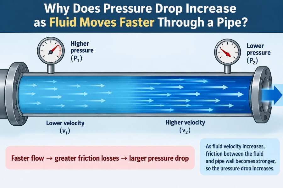

A shower that weakens when another tap opens, a pump that cannot deliver its expected flow, and a long process line that needs more energy than anticipated all point to the same engineering reality: moving fluid through a pipe costs pressure.
The effect can seem counterintuitive at first. A fast-moving fluid has more kinetic energy, so why does its measured pressure commonly fall along the pipe? The answer lies not in a single mechanism, but in the way flow exchanges energy with pipe walls, fittings, changes in elevation, and itself.
For chemical engineers, pressure drop is not just a hydraulic detail. It affects pump sizing, operating cost, heat-transfer performance, control-valve authority, product throughput, cavitation risk, and sometimes process safety.
The useful question is therefore more precise than “does faster flow reduce pressure?” It is: where does the pressure energy go as flow rate rises, and how quickly do the losses increase?
🚰 Pressure Is the Energy Available to Move Fluid
Pressure is force per unit area, but in flowing systems it is also a convenient measure of energy available per unit volume of fluid. A pressure difference between two locations supplies the driving force that pushes liquid or gas through a line.
If a pump raises liquid pressure upstream, fluid moves toward the lower-pressure downstream location. Along the way, some of that useful pressure energy may become fluid velocity, potential energy from elevation, or thermal energy through friction.
When engineers say “pressure drop,” they usually mean the reduction in static pressure between two specified points. The location matters: a pressure drop across 100 m of straight pipe is not the same as the pressure change across a nozzle or a pump.
🏃 Faster Flow Means Higher Velocity
For an incompressible liquid in a pipe of constant internal diameter, volumetric flow rate and average velocity are directly related:
Q = vAHere, Q is volumetric flow rate, v is average fluid velocity, and A is the pipe’s internal cross-sectional area. If the pipe size stays fixed, doubling the flow rate doubles the average velocity.
That simple relationship sets up the central issue. Wall friction and many local disturbances depend strongly on velocity, so a modest increase in throughput can require a much larger pressure difference.
🧱 Fluid Friction at the Pipe Wall
No real fluid slips perfectly along an ordinary pipe wall. Fluid immediately adjacent to the wall moves very slowly because of the no-slip condition, while fluid nearer the center travels faster.
Viscosity creates shear between neighboring layers moving at different speeds. The pump’s mechanical energy is gradually dissipated through this internal resistance, ultimately appearing as a very small temperature increase in the fluid and pipe surroundings.
The wall does not “consume” pressure as a material object might consume fuel. Rather, pressure energy is irreversibly converted into disordered microscopic motion. That irreversible conversion is called frictional loss or head loss.
📉 Why Frictional Loss Rises So Sharply
In many industrial pipe systems, flow is turbulent. Under turbulent conditions, pressure loss through a given pipe segment is approximately proportional to the square of velocity:
ΔP ∝ v²Since velocity is proportional to flow rate in a fixed pipe, pressure drop is often roughly proportional to flow rate squared. Increasing flow by 20% can therefore create a pressure drop increase closer to 44%, not 20%, when other conditions remain similar.
This is why a line that works comfortably at one production rate may become hydraulically restrictive at a higher rate. The relationship is nonlinear, and design margins can disappear quickly.
🌊 Laminar and Turbulent Flow Behave Differently
Not every flow follows the same velocity-squared pattern. In laminar flow, fluid moves in relatively orderly layers, with limited mixing between them. For fully developed laminar flow of a Newtonian fluid in a round pipe, pressure drop is proportional to velocity.
In turbulent flow, eddies and fluctuations transport momentum across the pipe. This creates substantially greater resistance, and the pressure-drop dependence commonly approaches a velocity-squared form.
| Flow regime | General behavior | Typical pressure-drop dependence |
|---|---|---|
| Laminar | Orderly viscous layers dominate | Approximately proportional to velocity |
| Transitional | Unstable mixture of behaviors | Less predictable; avoid relying on a simple rule |
| Turbulent | Eddies and wall roughness matter strongly | Often approximately proportional to velocity squared |
Many water-like fluids in plant piping operate turbulently. Highly viscous liquids, small tubing, and low flow rates may instead remain laminar.
🔢 Reynolds Number Identifies the Regime
The Reynolds number compares inertial effects with viscous effects:
Re = ρvD / μIn this expression, ρ is density, v is average velocity, D is internal diameter, and μ is dynamic viscosity. It is dimensionless, which makes it useful across fluids and equipment scales.
For flow in a smooth circular pipe, laminar flow is generally associated with Reynolds numbers below roughly 2,000, while clearly turbulent flow is often found above roughly 4,000. The region between is transitional, and real systems can shift behavior because of disturbances, fittings, or pulsation.
📐 The Darcy–Weisbach Framework
The most widely used general equation for frictional pressure drop in a straight, constant-diameter pipe is the Darcy–Weisbach equation:
ΔP = f(L/D)(ρv²/2)f is the Darcy friction factor, L is pipe length, D is internal diameter, and ρv²/2 is the dynamic-pressure term. The equation makes the main dependencies visible: pressure loss grows with length and density, falls with diameter, and responds strongly to velocity.
The friction factor is not a universal constant. It changes with Reynolds number and internal roughness. Reliable design therefore requires an appropriate correlation, chart, or validated hydraulic software model.
🌀 What Turbulence Adds to the Loss
Turbulence is not merely “fast flow.” It is a flow state characterized by irregular, three-dimensional velocity fluctuations. These fluctuations continually redistribute momentum between the fast central region and the slower wall region.
That mixing raises the rate at which energy is dissipated. It can also be useful: turbulence often improves heat and mass transfer, helps suspend solids, and reduces concentration gradients.
The design trade-off is clear. Higher velocity may improve mixing or heat-transfer coefficients, but it also raises pumping duty and can intensify vibration, erosion, and noise.
🪨 Pipe Roughness Becomes More Significant at High Flow
Even new pipe has microscopic surface irregularities. Corrosion, scale, deposits, weld beads, and aging can make the effective internal surface much rougher.
At low Reynolds number, viscosity can dominate so thoroughly that wall roughness has little influence. At high Reynolds number, turbulent eddies interact with surface projections, increasing drag and the friction factor.
For long-lived systems, assumed roughness deserves scrutiny. A line designed around clean, smooth pipe may not meet duty after fouling or corrosion reduces its hydraulic performance.
📏 Diameter Has an Outsized Effect
Pipe diameter affects pressure drop twice. A smaller diameter increases the ratio of length to diameter in Darcy–Weisbach, and it also forces the same flow rate through a smaller area, sharply increasing velocity.
For a given liquid flow rate in turbulent flow, a modest reduction in internal diameter can cause a major rise in pressure loss. This is why nominal pipe size alone is insufficient: wall thickness, schedule, lining, and deposits all alter the true internal diameter.
Choosing a larger pipe can reduce operating energy, but it increases capital cost and may reduce velocity below values needed for solids transport or self-cleaning service. There is no universally “best” diameter.
🛣️ Long Pipes Accumulate Losses
Every meter of straight pipe contributes some frictional loss. A short section may be negligible, but a transfer line running across a plant or between storage tanks can consume a substantial fraction of the available pump head.
Length matters linearly in the Darcy–Weisbach expression. Doubling the straight-pipe length approximately doubles its frictional pressure drop when flow conditions and diameter are unchanged.
This is why routing matters during layout. A compact route with sensible equipment placement may lower both installed piping cost and lifetime pumping energy.
🔩 Fittings Create Minor Losses That May Not Be Minor
Elbows, tees, valves, reducers, entrances, exits, strainers, meters, and partially open control valves disturb the velocity pattern. Flow separates, swirls, recirculates, or accelerates through these features, creating additional irreversible losses.
These are traditionally called minor losses, but the phrase can mislead. In a short, fitting-dense skid, losses through valves and fittings can exceed losses in the straight pipe.
A common calculation form is:
ΔP = K(ρv²/2)The loss coefficient K depends on component geometry and condition. Manufacturer data are often more appropriate than generic values for specialized valves, filters, and proprietary equipment.
↪️ Bends Are Not All Hydraulically Equal
A gradual long-radius elbow generally produces less loss than a tight elbow because the fluid changes direction more smoothly. A sharp turn encourages separation and secondary circulation, which dissipate energy.
Likewise, two elbows placed close together can interact. The flow may enter the second fitting already distorted by the first, especially when they are in different planes.
Good piping layout does not mean eliminating every bend. It means recognizing that geometry affects hydraulic resistance and reserving tight, crowded routing for cases where space constraints justify it.
🔻 Contractions, Expansions, and Nozzles
When a pipe narrows, velocity rises in the smaller section. Some static pressure is converted to kinetic energy, and additional energy is lost if the contraction is abrupt.
When a pipe expands, velocity falls and some kinetic energy can be recovered as static pressure. However, a sudden expansion often causes flow separation and turbulence, so recovery is incomplete.
This distinction is essential: a lower static pressure at a narrow point is not automatically all “friction loss.” Part may be a reversible exchange between pressure and velocity. The irreversible portion comes from viscous and turbulent dissipation.
⚖️ Bernoulli’s Equation Needs a Real-World Correction
The ideal Bernoulli equation relates pressure, velocity, and elevation for an ideal fluid with no friction. In practical piping, engineers use an extended energy balance that includes pumps, turbines, and losses.
P₁/(ρg) + v₁²/(2g) + z₁ + h_p = P₂/(ρg) + v₂²/(2g) + z₂ + h_L + h_tHere, h_p is pump head added, h_t is turbine head removed, and h_L represents head loss. This form prevents a common mistake: applying ideal Bernoulli to a real pipe and concluding that pressure changes only because velocity changes.
For equal-diameter horizontal pipe, average velocity is similar at both ends. Any sustained pressure decrease along that pipe is primarily evidence of frictional and local losses.
⛰️ Elevation Changes Are a Separate Pressure Effect
If liquid flows uphill, pressure must also support the gain in gravitational potential energy. For downhill flow, gravity contributes energy and can offset part of the frictional loss.
Elevation is independent of whether velocity rises. A vertical riser can show a substantial pressure reduction even at low velocity, while a horizontal line can show frictional pressure drop without any elevation change.
Separating these effects is especially important in tall columns, tank farms on uneven terrain, and pipeline systems. A pressure profile is meaningful only when the elevations of the measurement points are known.
💨 Gases Require Extra Care
Gas density can change appreciably as pressure falls, particularly across long lines, restrictions, compressors, and high-pressure systems. As gas expands, its velocity may increase even when the mass flow rate is constant.
That coupling makes gas pressure-drop calculations more complex than incompressible liquid calculations. Temperature changes, compressibility, sonic-flow limits, and the equation of state can all matter.
Using a liquid-style calculation with a single fixed density may be acceptable only when density change is demonstrably small. Otherwise, use a compressible-flow method appropriate to the pressure range and gas composition.
🧴 Viscosity Can Transform the Hydraulic Problem
Viscosity measures a fluid’s resistance to deformation. Honey flows more reluctantly than water because its viscosity is much higher; many oils, polymer solutions, slurries, and cold process liquids behave similarly.
Higher viscosity reduces Reynolds number at a given velocity and can push a system toward laminar flow. In laminar flow, viscosity directly governs the pressure drop, and temperature changes can have dramatic hydraulic consequences.
For temperature-sensitive liquids, a line may start easily when warm but become difficult to pump after cooling. Heat tracing, insulation, shorter routes, larger pipes, or different pumping arrangements may be needed.
🧪 Non-Newtonian Fluids Do Not Follow the Simplest Rules
Newtonian fluids have a viscosity that is essentially independent of shear rate. Water and many simple hydrocarbons approximate this behavior. Many process fluids do not.
Shear-thinning fluids, such as some polymer solutions and food products, become less viscous at higher shear rates. Shear-thickening materials do the opposite. Yield-stress fluids may resist flow until a threshold stress is exceeded.
These materials need rheological data and specialized pressure-drop correlations. Treating them as Newtonian with one convenient viscosity can lead to serious errors in pump sizing, startup planning, and line-cleaning design.
🧱 Slurries Add Solids-Related Risks
A slurry carries solid particles in a liquid. Pressure drop may be higher than for the carrier liquid because energy is needed to move particles and because solids alter turbulence and effective viscosity.
Velocity cannot always be minimized to save pumping power. If it becomes too low, particles may settle, creating deposition, blockage, unstable restart conditions, or severe local wear after flow resumes.
Conversely, excessive velocity can accelerate erosion at elbows, reducers, valves, and pump components. Slurry line design balances pressure loss against deposition and erosion risks using data for the actual solids and concentration.
🔧 Pumps Must Supply the Required Head
A pump must provide enough head to overcome static elevation, frictional losses, local losses, and any required downstream pressure. As flow rises, system friction rises, so the required pump head usually rises as well.
The point where the pump curve intersects the system curve is the operating point. Changing valve position, pipe roughness, fluid viscosity, or pump speed shifts one or both curves.
A pump selected only for a nominal design flow may operate poorly when conditions vary. Engineers check the expected operating range, efficiency, available suction head, minimum-flow needs, and mechanical limits.
🫧 Low Pressure Can Lead to Cavitation
If local liquid pressure falls below vapor pressure, vapor bubbles may form. If those bubbles subsequently enter a higher-pressure region and collapse, the phenomenon is called cavitation.
Cavitation can create noise, vibration, loss of pump performance, and damage over time. It is particularly relevant at pump suction, in control valves, across restrictions, and at high-velocity locations.
Pressure-drop calculations help identify vulnerable points, but vapor pressure depends strongly on temperature and composition. A warm volatile liquid needs a more careful assessment than cool water under similar piping geometry.
🎛️ Control Valves Intentionally Spend Pressure
A control valve regulates flow by creating a variable restriction. Its pressure drop is not always undesirable; it provides the controllable resistance needed to adjust the process flow.
Problems arise when piping consumes too much of the available pressure drop. Then the valve has little authority: moving it produces only a weak change in flow. If the valve consumes nearly all available pressure, it may operate near a very closed position and become sensitive, noisy, or prone to cavitation.
Good control design allocates pressure drop across the system deliberately rather than treating the valve as an afterthought.
📊 A Simple Hypothetical Example
Imagine water flowing through the same horizontal pipe at two operating rates. If the flow is turbulent and the first rate produces an average velocity of 1 m/s, increasing that velocity to 2 m/s approximately quadruples the dynamic-pressure term, ρv²/2.
The exact pressure-drop increase will not always be exactly four because the friction factor can change with Reynolds number. Still, the example captures the practical message: doubling liquid flow in a turbulent line often requires far more than double the friction-driving pressure difference.
Now imagine a pump with limited spare head. The higher rate may be impossible without changing the pump, opening restrictions, or increasing pipe diameter.
🧮 Measure the Right Pressures in the Right Places
Pressure instruments provide useful data only when their locations and reference elevations are understood. A gauge immediately upstream of an elbow and one downstream of a control valve do not isolate straight-pipe friction.
For a meaningful test, record flow rate, fluid temperature, pressure at clearly defined points, elevations, valve positions, and the state of filters or strainers. Temperature matters because density and viscosity may change.
Differential-pressure transmitters are particularly useful across filters, heat exchangers, packed beds, and selected pipe sections. A rising differential pressure at constant flow can signal fouling, blockage, or an unintended restriction.
🧹 Fouling Changes Pressure Drop Over Time
Scale, wax, biological growth, polymer buildup, corrosion products, and solids deposits reduce the effective bore and roughen the surface. Both changes increase hydraulic resistance.
The operational clue is often a growing pressure drop at the same flow rate or a declining flow rate at the same pump conditions. The trend can be more informative than a single reading.
Cleaning schedules should consider process consequences, not just elapsed time. Unnecessary cleaning costs money, while delayed cleaning can restrict production or push equipment into unfavorable operating conditions.
⚠️ Common Calculation Mistakes
Pressure-drop estimates are only as trustworthy as their inputs and assumptions. Several errors appear repeatedly in preliminary calculations and troubleshooting work.
- Using nominal diameter instead of the actual internal diameter.
- Ignoring fittings, filters, valves, meters, and partially closed isolation valves.
- Mixing Darcy and Fanning friction factors; the Darcy value is four times the Fanning value.
- Assuming water properties for a viscous, hot, chilled, multiphase, or composition-changing process fluid.
- Treating a compressible gas as incompressible over a large pressure change.
- Applying a clean-pipe roughness value to an old or fouled system without checking performance data.
A transparent calculation that states its assumptions is generally more useful than a highly precise-looking result based on unsuitable inputs.
🛠️ Ways to Reduce Excessive Pressure Drop
The right solution depends on why the loss is high. Increasing pipe diameter is powerful for a new installation, but may be expensive or impractical for an existing plant.
- Remove unnecessary restrictions and replace unsuitable fittings with lower-loss designs.
- Clean or replace fouled strainers, filters, exchangers, and piping where deposits are confirmed.
- Use smoother routing and larger-radius bends where layout changes are possible.
- Reduce viscosity through controlled heating when product quality and safety allow.
- Use parallel lines or staged pumping when a single line cannot carry the required flow efficiently.
- Review operating flow targets; lower velocity may be preferable if throughput requirements permit.
Each option has trade-offs involving capital cost, energy use, maintainability, controllability, and process constraints.
🧭 Design Velocity Is a Decision, Not a Universal Rule
Engineers often use velocity ranges as screening guides, but there is no single correct velocity for all services. A clean, low-viscosity liquid, a corrosive chemical, a gas, a slurry, and a viscous polymer solution demand different priorities.
Low velocity usually reduces frictional loss but may permit settling, stratification, poor heat transfer, or long residence time. High velocity can shrink pipe size and improve suspension or transfer rates, but increases pumping power, noise, vibration, and erosion potential.
The best choice emerges from a complete process and lifecycle assessment, not from pressure drop alone.
🧠 The Core Principle to Remember
Faster fluid motion requires a larger pressure difference because the system must overcome stronger viscous and turbulent resistance. In a fixed pipe carrying turbulent flow, the resulting frictional pressure loss commonly increases approximately with the square of velocity.
Pipe length, internal diameter, roughness, fittings, fluid density, viscosity, elevation, and compressibility determine how that principle appears in a real installation. Pressure can also be converted temporarily into velocity or elevation, so engineers must distinguish those reversible energy changes from irreversible losses.
Pressure drop is the hydraulic price of moving a real fluid through a real system—and that price rises rapidly when velocity rises.
Once pressure loss is viewed as an energy balance rather than a mysterious disappearance of pressure, pipe sizing, pump selection, troubleshooting, and process optimization become much easier to reason through. 🧪🚰📈