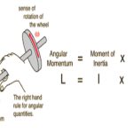
Assume that F and M derive from two types of forces, namely, body forces f, such as gravitational attractions—defined such that force fdV acts on volume element dV (see Figure 1)—and surface forces, which represent the mechanical effect of matter immediately adjoining that along the surface S of the volume V being considered. Cauchy formalized in 1822 a basic assumption of continuum mechanics that such surface forces could be represented as a stress vector T, defined so that TdS is an element of force acting over the area dS of the surface (Figure 1). Hence, the principles of linear and angular momentum take the forms.
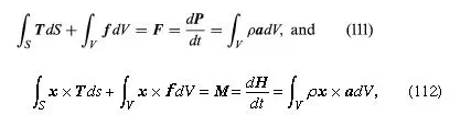
which are now assumed to hold good for every conceivable choice of region V. In calculating the right-hand sides, which come from dP/dt and dH/dt, it has been noted that ρdV is an element of mass and is therefore time-invariant; also, a = a(x, t) = dv/dt is the acceleration, where the time derivative of v is taken following the motion of a material point so that a(x, t)dt corresponds to the difference between v(x + vdt, t + dt) and v(x, t). A more detailed analysis of this step shows that the understanding of what TdS denotes must now be adjusted to include averages, over temporal and spatial scales that are large compared to those of microscale fluctuations, of transfers of momentum across the surface S due to the microscopic fluctuations about the motion described by the macroscopic velocity v.
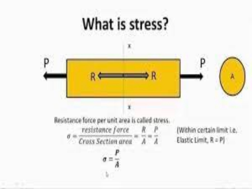
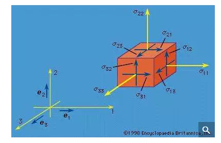
The nine quantities σij(i, j = 1, 2, 3) are called stress components; these will vary with position and time—i.e., σij = σij(x, t)—and have the following interpretation. Consider an element of surface dS through a point x with dS oriented so that its outer normal (pointing away from the region V, bounded by S) points in the positive xi direction, where i is any of 1, 2, or 3. Then σi1, σi2, and σi3 at x are defined as the Cartesian components of the stress vector T (called T(i)) acting on this dS. Figure 2 shows the components of such stress vectors for faces in each of the three coordinate directions. To use a vector notation with e1, e2, and e3 denoting unit vectors along the coordinate axes (Figure 2), T(i) = σi1e1 + σi2e2 + σi3e3. Thus, the stress σij at x is the stress in the j direction associated with an i-oriented face through point x; the physical dimension of the σij is [force]/[length]2. The components σ11, σ22, and σ33 are stresses directed perpendicular, or normal, to the face on which they act and are normal stresses; the σij with i ≠ j are directed parallel to the face on which they act and are shear stresses.
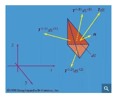
By hypothesis, the linear momentum principle applies for any volume V. Consider a small tetrahedron (Figure 3) at x with an inclined face having an outward unit normal vector n and its other three faces oriented perpendicular to the three coordinate axes. Letting the size of the tetrahedron shrink to zero, the linear momentum principle requires that the stress vector T on a surface element with outward normal n be expressed as a linear function of the σij at x. The relation is such that the j component of the stress vector T is Tj = n1σ1j + n2σ2j + n3σ3j for (j = 1, 2, 3). This relation for T (or Tj) also demonstrates that the σij have the mathematical property of being the components of a second-rank tensor.
Suppose that a different set of Cartesian reference axes 1′, 2′, and 3′ have been chosen. Let x1′, x2′, and x3′ denote the components of the position vector of point x and let σkl′(k, l = 1, 2, 3) denote the nine stress components relative to that coordinate system. The σkl′ can be written as the 3 × 3 matrix [σ′], and the σij as the matrix [σ], where the first index is the matrix row number and the second is the column number. Then the expression for Tj implies that [σ′] = [α][σ][α]T, which is the defining equation of a second-rank tensor. Here [α] is the orthogonal transformation matrix, having components αpq = ep′ · eq for p, q = 1, 2, 3 and satisfying [α]T[α] = [α][α]T = [I], where the superscript T denotes transpose (interchange rows and columns) and [I] denotes the unit matrix, a 3 × 3 matrix with unity for every diagonal element and zero elsewhere; also, the matrix multiplications are such that if [A] = [B][C], then Aij = Bi1C1j + Bi2C2j + Bi3C3j.