
A process unit can look perfectly healthy from the outside: pumps are running, temperature is on target, and flow is close to plan. Yet conversion may fall, a separator may carry liquid into a gas line, or a treatment system may miss its effluent limit.
Often, the missing clue is not a temperature or a pressure. It is time: how long material actually remains inside the equipment.
A tank holding 10 m³ and receiving 2 m³/h appears to offer five hours of residence time. That simple calculation is useful, but it does not automatically mean every molecule spends five hours in the tank. Some material may bypass the active zone, some may recirculate, and some may remain nearly stagnant.
Residence time connects equipment size, flow rate, reaction rate, mixing, separation, quality, and safety. Understanding it turns a basic volume-flow calculation into a practical tool for diagnosing and designing process equipment.
⏱️ What Residence Time Means
Residence time is the time a parcel of material spends within a defined piece of equipment or process zone. It applies to liquids, gases, solids, slurries, and even to a particular phase within multiphase equipment.
The term may refer to an average value, an ideal design value, or the full spread of times experienced by different fluid elements. Those distinctions matter because real equipment rarely behaves as an ideal vessel.
🧮 The Fundamental Volume-Flow Relationship
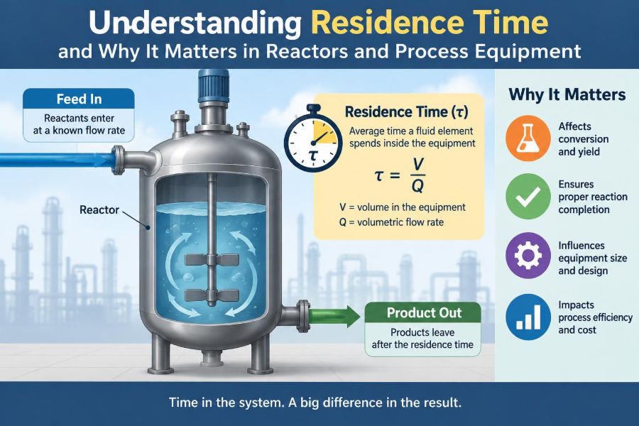
For a vessel at steady state, the nominal or hydraulic residence time is commonly written as τ = V/Q, where τ is residence time, V is the relevant hold-up volume, and Q is volumetric flow rate.
If a liquid volume of 6 m³ is held in a vessel with a liquid outlet flow of 1.5 m³/h, the nominal residence time is 4 h. Units must be consistent: litres with litres per minute, or cubic metres with cubic metres per hour.
This equation is a material balance result, not a guarantee about the path of each particle. It is best viewed as the starting point for engineering judgment.
🚰 Why “Active Volume” Matters More Than Vessel Volume
The relevant V is usually not the nameplate volume of a tank. It is the working or active volume: the volume occupied by the material of interest under normal operating conditions.
Freeboard above a liquid level is not liquid residence volume. Neither is a dead pocket below an outlet that does not exchange effectively. In a gas-liquid separator, liquid and gas each require their own hold-up and flow basis.
Level changes can therefore change residence time substantially. A level controller that operates at a lower set point may reduce liquid residence time even when inlet flow has not changed.
⚖️ Steady State Makes the Simple Calculation Valid
At steady state, vessel inventory is constant, so average inlet and outlet flow rates match for the conserved material basis. This is the condition under which τ = V/Q is most directly useful.
During startup, shutdown, batch filling, grade changes, or level disturbances, inventory changes with time. A single residence-time number then becomes less representative, and a dynamic material balance is often needed.
For compressible gases, pressure and temperature changes also alter volumetric flow. Engineers should state whether flow is actual operating volume or a standardized reference volume.
🧭 Mean Residence Time Is an Average, Not a Promise
The mean residence time is the average time material spends in a system. It is especially useful for mass balances, preliminary sizing, and comparing operating conditions.
Imagine 100 small fluid parcels entering a vessel. If some leave quickly and others remain much longer, their average can still equal the nominal τ. A process sensitive to the earliest material leaving may perform poorly despite an acceptable average.
This is why a mean value alone is insufficient for many reactors, sterilization systems, contactors, and separation devices.
📈 Residence Time Distribution Reveals the Real Flow Pattern
A residence time distribution, usually abbreviated RTD, describes the fraction of material leaving at each time after entering a system. It captures the spread around the mean residence time.
RTD is often measured by injecting a detectable tracer at the inlet and monitoring its concentration at the outlet. Salt conductivity, dyes, or other compatible tracers may be used depending on the process and instrumentation.
A narrow RTD indicates that parcels experience relatively similar contact times. A broad RTD signals a wider mix of fast and slow paths, which can affect conversion, product consistency, and contaminant removal.
➡️ Plug Flow Is the Ideal of Ordered Movement
In ideal plug flow, fluid moves through a pipe or tubular reactor as orderly slices. Each slice has the same residence time, with no axial mixing between slices.
A long, well-designed tubular reactor can approach plug-flow behavior, particularly when flow is turbulent enough to mix across the pipe radius while limiting mixing along its length. Real tubes still show dispersion due to velocity profiles, bends, fittings, and diffusion.
Plug flow is attractive for many reactions because reactants enter at their highest concentration and progress continuously along the reactor length.
🌀 Complete Mixing Is the Other Classic Ideal
An ideal continuous stirred-tank reactor, or CSTR, is completely mixed. Its contents have the same composition and temperature everywhere, and the outlet has that same condition.
Some material entering a perfectly mixed tank can, in theory, appear at the outlet very soon afterward. Other material remains much longer. Its RTD is broad even though the average residence time remains V/Q.
Real agitated tanks are not automatically ideal CSTRs. Baffles, impeller position, liquid height, viscosity, feed location, and outlet placement all influence mixing.
🔄 Tanks in Series Can Approximate Better Flow Behavior
Connecting several mixed tanks in series narrows the RTD compared with one large mixed tank of the same total volume. Each stage reduces the degree to which freshly entering material can immediately reach the final outlet.
This model is useful for staged neutralization, biological treatment, extraction, and some reaction systems. More tanks generally move behavior toward plug flow, but extra vessels add cost, controls, maintenance, and pressure drop.
The appropriate number of stages depends on kinetics and process sensitivity, not on a universal rule.
🕳️ Dead Zones Reduce Effective Contact
A dead zone is a region with weak exchange with the main flowing stream. Material in that region can remain for a long time while contributing little to useful reaction, heat transfer, or mixing.
Dead zones may occur behind internals, in vessel corners, beneath poorly designed agitators, around coils, or in large tanks with insufficient circulation. They can also accumulate solids, creating cleaning and contamination concerns.
A vessel can have a long apparent hold-up time while offering less useful active contact than expected. This is one reason nominal residence time should not be mistaken for process performance.
⚡ Short-Circuiting Creates Fast Exit Paths
Short-circuiting occurs when inlet material reaches the outlet through an unusually direct path. It is common when nozzles are poorly located or when internal flow guidance is absent.
In a clarifier, short-circuiting can reduce settling opportunity. In a reactor, it can send under-reacted feed downstream. In a storage tank, it can make a concentration change appear sooner than a well-mixed model predicts.
Inlet diffusers, baffles, calming zones, and better outlet design can reduce this problem, but each modification should be evaluated for fouling, cleanability, and hydraulic effects.
🧪 Residence Time and Chemical Reaction Conversion
Reactants need sufficient time under suitable conditions to reach the desired conversion. In a continuous reactor, residence time is therefore a central design variable alongside temperature, pressure, catalyst activity, and feed composition.
For a hypothetical slow reaction, increasing τ by reducing flow or increasing active volume may increase conversion. But the benefit depends on reaction kinetics. A reaction with a high rate at the beginning may need a different reactor arrangement than one that proceeds gradually.
Longer residence time is not inherently better. It can increase side reactions, polymer degradation, catalyst deactivation exposure, or energy consumption.
🌡️ Temperature Profiles Can Change the Needed Time
Reaction rates are often strongly temperature-dependent. A reactor may have enough nominal residence time at its design temperature but become conversion-limited when heat removal, heating duty, or feed temperature changes.
Temperature nonuniformity can be equally important. Hot zones may accelerate unwanted reactions, while cold zones may leave material under-reacted even when the average temperature looks acceptable.
Residence time and heat transfer must be considered together. A long hold-up with poor thermal control is not a reliable substitute for a properly designed reactor.
🧫 Bioreactors Need Time for Biological Work
In fermentation and wastewater treatment, residence time affects how long microorganisms and substrates remain in contact. However, the relevant time can differ for liquid, gas, and biomass.
For systems that retain cells using membranes, settling, or attached growth, the solids retention time may be much longer than the liquid hydraulic residence time. This distinction is fundamental: biomass can remain active even as water moves through comparatively quickly.
Biological systems also respond to oxygen transfer, nutrients, pH, toxicity, and temperature. Hydraulic residence time alone cannot predict treatment performance.
💧 Separators Need Enough Time for Phases to Disengage
Gravity separators rely on density differences. Droplets or particles need time to rise, settle, coalesce, or otherwise separate before the continuous phase exits.
For example, an oil-water separator may have an adequate liquid residence time on paper but still perform poorly if droplets are too small, turbulence is high, or the interface level is unstable. Residence time is necessary, but settling velocity and hydraulic design determine whether it is sufficient.
Gas-liquid separators likewise require appropriate vapor velocity and liquid hold-up. Excessive gas velocity can entrain droplets regardless of nominal vessel volume.
🧱 Solids Make the Picture More Complicated
Slurries, powders, fluidized beds, and granular systems can show different residence times for solids and fluids. A liquid may flow through a vessel while dense particles settle or recirculate, producing a much longer solids residence time.
In a fluidized catalytic process, the catalyst circulation rate and inventory help determine catalyst contact time, while gas residence time follows a different path. Treating both phases as one homogeneous stream can lead to poor interpretations.
Particle size distribution, segregation, attrition, and buildup can all change solids hold-up over time.
🛢️ Storage Tanks Also Have Residence-Time Behavior
Storage is often viewed as simple inventory management, but residence time affects blend uniformity, product age, additive distribution, and degradation risk. A tank may operate as a mixed tank, a stratified vessel, or something between those extremes.
For sensitive products, long residence time can promote oxidation, settling, phase separation, or loss of volatile components. For blending operations, too little time may leave composition nonuniform.
Recirculation can improve uniformity, but it also adds pump energy, shear, heat input, and possible entrainment.
🏭 Pipeline Residence Time Matters During Transitions
A pipeline has a residence time based on its internal volume and actual flow rate. This becomes critical during product changeovers, cleaning, chemical dosing, and analyzer response interpretation.
A control action at an upstream point cannot affect a downstream analyzer until material has traveled through the line. Long transport delay can make feedback control sluggish or unstable if the controller is tuned as though the response were immediate.
Dead legs and low-flow branches may retain old material much longer than the main line, creating quality or contamination problems.
📏 Space Time Is Closely Related but Not Always Identical
In reactor engineering, space time is commonly defined as reactor volume divided by inlet volumetric flow rate. Under steady-state, constant-density conditions, it is numerically similar to mean residence time.
The terms diverge when density changes substantially, phases have different hold-ups, flow is compressible, or volume and flow are defined at different conditions. Gas-phase reactions with changing mole number are a familiar example.
Clear reporting prevents confusion: state the basis, location, temperature, pressure, and whether the stated volume is total, liquid, gas, or catalyst bed volume.
📊 A Practical Comparison of Common Flow Models
| Model or condition | Residence-time behavior | Typical implication |
|---|---|---|
| Ideal plug flow | Nearly all material has the same residence time | Predictable progression along a tube or packed bed |
| Ideal CSTR | Broad distribution, with some early exit | Uniform tank composition but less ordered contact |
| Tanks in series | Intermediate distribution that narrows with more stages | Useful approximation for staged processes |
| Dead zones | Long tail of retained material | Inactive volume, fouling, or slow washout risk |
| Short-circuiting | Early tracer breakthrough | Insufficient contact for some of the feed |
🎨 Tracer Tests Turn Assumptions into Evidence
Tracer testing is one of the most practical ways to investigate actual residence-time behavior. A carefully selected tracer is introduced at the inlet, and outlet concentration is recorded over time.
A pulse input can reveal the full response curve. A step change, such as switching to a known tracer concentration, can be easier to implement and interpret for some systems.
The tracer must be compatible with the process, detectable at suitable concentrations, and unlikely to react, adsorb, separate into another phase, or alter process behavior. Safety and disposal requirements also matter.
📉 Reading a Tracer Response Curve
An early outlet response suggests bypassing or short-circuiting. A delayed and broad peak can indicate dispersion, mixing, or a range of flow paths. A long tail often points to stagnant regions, adsorption, or slow exchange zones.
The area under a properly normalized outlet curve relates to tracer recovery. Poor recovery may mean sampling errors, unaccounted outlets, tracer loss, or a tracer that does not follow the same path as the material being studied.
Interpretation should not jump from one curve shape to one physical cause. Several mechanisms can produce similar-looking responses, so process knowledge and additional measurements remain essential.
🔍 Flow Rate Changes Directly Change Residence Time
With fixed active volume, residence time is inversely proportional to flow rate. Doubling Q halves nominal τ. This simple relationship is valuable for quickly assessing the effect of throughput changes.
In real equipment, changing flow also changes hydrodynamics. Higher flow can increase turbulence and improve mixing in one unit while causing entrainment, channeling, or pressure-drop problems in another.
Do not assume that scaling flow changes only time. It may change the entire flow pattern.
🧼 Fouling and Level Control Quietly Alter Hold-Up
Fouling can reduce available volume in pipes, packed beds, filters, and vessels. Deposits may also create preferential channels or stagnant pockets, changing the RTD in opposite directions within the same unit.
Level-control changes can alter liquid hold-up, while interface-control problems can change the effective volume available to each phase. These shifts may be gradual and easy to miss in routine operations.
Trend data for level, differential pressure, flow, and product quality can help identify when a previously valid residence-time assumption no longer represents the equipment.
🧰 Design Levers for Adjusting Contact Time
Engineers can change residence time through vessel volume, operating level, throughput, parallel or series arrangement, recycle, and internal design. The best choice depends on what is limiting performance.
- Increase active volume when more sustained contact is genuinely required.
- Reduce flow when capacity allows and slower passage improves the outcome.
- Use staged vessels when reduced back-mixing benefits reaction or treatment.
- Improve internals or nozzle placement when bypassing is the main problem.
- Add recycle only when its mixing, energy, and control consequences are understood.
A larger vessel is not always the best remedy. If short-circuiting dominates, improving flow distribution may produce more useful contact than simply adding volume.
⚠️ Safety Implications of Long and Short Residence Times
Residence time can influence safety in several directions. Too short a time can leave reactive intermediates, dissolved gas, or contaminants insufficiently treated. Too long a time can allow accumulation, thermal degradation, unwanted reaction, or loss of inhibitor effectiveness.
For exothermic systems, hold-up affects how much reacting material is present during an upset. A larger inventory can provide more process buffering but may also increase the energy available for a runaway scenario.
Safety assessment requires reaction hazards, relief design, operating procedures, and credible upset scenarios. Residence time is one important input, not a stand-alone safety conclusion.
🧑🔧 Common Calculation Mistakes
Many errors come from using a correct equation with an inappropriate basis. A quick review can prevent misleading results.
- Using total vessel capacity instead of normal working volume.
- Mixing actual and standard gas volumetric flow rates.
- Ignoring separate phase hold-ups in multiphase equipment.
- Using design flow when the question concerns current operation.
- Assuming nominal residence time represents minimum contact time.
- Forgetting recirculation, bypass lines, or parallel flow paths.
- Reporting a result without units or operating conditions.
📝 A Reliable Workflow for Everyday Calculations
Start by defining the system boundary: is the question about a vessel, a liquid zone, a packed bed void space, or a whole process train? Then identify the material phase and the operating condition of interest.
- Determine the active hold-up volume, not merely equipment capacity.
- Use the corresponding inlet or outlet flow at the same temperature and pressure basis.
- Calculate τ = V/Q for a steady-state nominal value.
- Ask whether mixing, bypassing, phase separation, or reaction makes an RTD assessment necessary.
- Compare the result with the process requirement: conversion, settling, blending, delay, or safety margin.
This workflow keeps the arithmetic simple while ensuring the result answers the actual engineering question.
🧠 Choosing the Right Level of Model Detail
A spreadsheet calculation may be entirely adequate for preliminary tank sizing or estimating a transport delay. A detailed RTD study, computational fluid dynamics model, or dynamic simulation may be justified when poor distribution has significant quality, environmental, production, or safety consequences.
More detailed models are not automatically more useful. They need reliable geometry, operating data, and assumptions. A sophisticated simulation built on uncertain flow conditions can create false confidence.
Use the simplest model that captures the decision-critical behavior, then validate it with operating evidence where practical.
🔗 The Core Principle: Time Must Match the Process Need
Residence time is not simply a number calculated from volume and flow. It is the link between the physical route material takes and the time-dependent work the process must accomplish.
For reaction, the question is whether material has enough time at the right temperature and composition. For separation, it is whether droplets or particles have time to disengage under the real hydraulic conditions. For control, it is whether transport delay has been recognized. For storage, it is whether age and mixing suit the product.
The strongest engineering decisions combine nominal residence time with active volume, flow pattern, phase behavior, and the specific performance objective.
Calculate the average, investigate the distribution when performance depends on it, and always define what “time in the equipment” truly means for the process. 🧪⏱️🏭