In the mixing of solid particles, the following three mechanisms may be involved:
A. Convective mixing, in which groups of particles are moved from one position to another,
B. Diffusion mixing, where the particles are distributed over a freshly developed interface, and
C. Shear mixing, where slipping planes are formed.
These mechanisms operate to varying extents in different kinds of mixers and with different kinds of particles. A trough mixer with a ribbon spiral involves almost pure
convective mixing, and a simple barrel-mixer involves mainly a form of diffusion mixing. The mixing of pastes is discussed in the section on Non-Newtonian Technology in
Volume 1, Chapter 7.
The degree of mixing
It is difficult to quantify the degree of mixing, although any index should be related to the properties of the required mix, should be easy to measure, and should be suitable for a variety of different mixers. When dealing with solid particles, the statistical variation in composition among samples withdrawn at any time from a mix is commonly used as a measure of the degree of mixing. The standard deviation s (the square root of the mean of the squares of the individual deviations) or the variance s2 is generally used. Aparticulate material cannot attain the perfect mixing that is possible with two fluids, and the best that can be obtained is a degree of randomness in which two similar particles may well be side by side. No amount of mixing will lead to the formation of a uniform mosaic as shown in Figure 1.17, but only to a condition, such as shown in Figure 1.18,
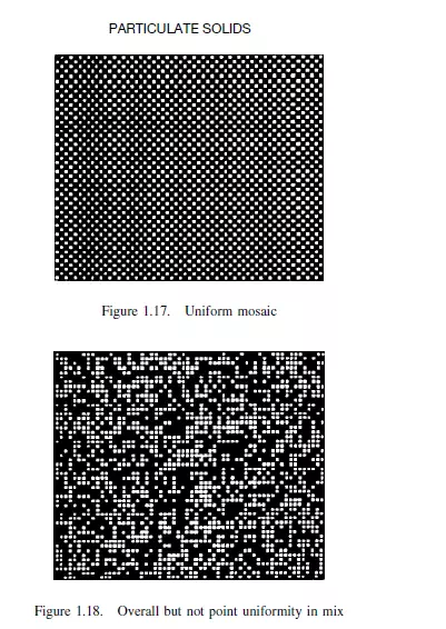
where there is an overall uniformity but not point uniformity. For a completely random mix of uniform particles distinguishable, say, only by colour, LACEY(18,19) has shown that:

where s2 r is the variance for the mixture, p is the overall proportion of particles of one colour, and n is the number of particles in each sample. This equation illustrates the importance of the size of the sample in relation to the size of the particles. In an incompletely randomised material, s2 will be greater, and in a completely unmixed system, indicated by the suffix 0, it may be shown that:

which is independent of the number of particles in the sample. Only a definite number of samples can in practice be taken from a mixture, and hence s will itself be subject to
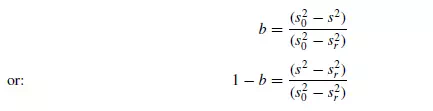
random errors. This analysis has been extended to systems containing particles of different sizes by BUSLIK(20). When a material is partly mixed, then the degree of mixing may be represented by some term b, and several methods have been suggested for expressing b in terms of measurable quantities. If s is obtained from examination of a large number of samples then, as suggested by Lacey, b may be defined as being equal to sr/s, or (s0 − s)/(s0 − sr ), as suggested by KRAMERS(21) where, as before, s0 is the value of s for the unmixed material. This form of expression is useful in that b = 0 for an unmixed material and 1 for a completely randomised material where s = sr. If s2 is used instead of s, then this expression may be modified to give:
For diffusive mixing, b will be independent of sample size provided the sample is small. For convective mixing, Kramers has suggested that for groups of particles randomly
distributed, each group behaves as a unit containing ng particles. As mixing proceeds ng becomes smaller. The number of groups will then be np/ng, where np is the number of particles in each sample. Applying equation 1.33:
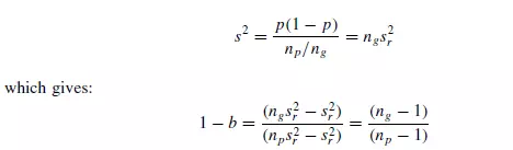
Thus, with convective mixing, 1 − b depends on the size of the sample.
Example
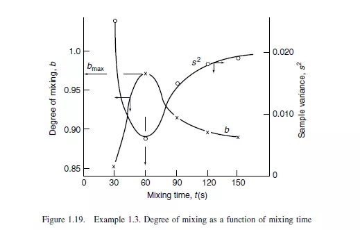
The performance of a solids mixer was assessed by calculating the variance occurring in the mass fraction of a component amongst a selection of samples withdrawn from the mixture. The quality was tested at intervals of 30 s and the data obtained are:
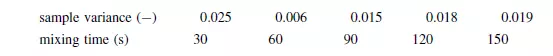
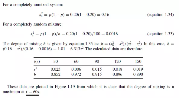
If the component analysed represents 20 per cent of the mixture by mass and each of the samples removed contains approximately 100 particles, comment on the quality of the mixture produced and present the data in graphical form showing the variation of the mixing index with time.
Solution
The rate of mixing
Expressions for the rate of mixing may be developed for any one of the possible mechanisms. Since mixing involves obtaining an equilibrium condition of uniform randomness, the relation between b and time might be expected to take the general form:

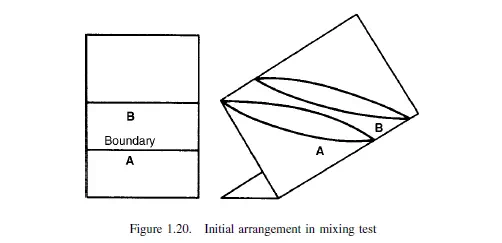
where c is a constant depending on the nature of the particles and the physical action of the mixer. Considering a cylindrical vessel (Figure 1.20) in which one substance A is poured into the bottom and the second B on top, then the boundary surface between the two materials is a minimum. The process of mixing consists of making some of A enter the space occupied by B, and some of B enter the lower section originally filled by A. This may be considered as the diffusion of A across the initial boundary into B, and of B into A. This process will continue until there is a maximum degree of dispersion, and a maximum interfacial area between the two materials. This type of process is somewhat akin to that of diffusion, and tentative use may be made of the relationship given by Fick’s law discussed in Volume 1, Chapter 10. This law may be applied as follows.
If a is the area of the interface per unit volume of the mix, and am the maximum interfacial surface per unit volume that can be obtained, then:

It is assumed that, after any time t , a number of samples are removed from the mix, and examined to see how many contain both components. If a sample contains both
components, it will contain an element of the interfacial surface. If Y is the fraction of the samples containing the two materials in approximately the proportion in the whole
mix, then:

a) the total volume of the material,
b) the inclination of the drum,
c) the speed of rotation of the drum,
d) the particle size of each component,
e) the density of each component, and
f) the relative volume of each component.
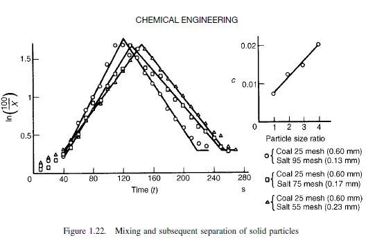
Whilst the precise values of c are only applicable to the particular mixer under examination, they do bring out the effect of these variables. Thus, Figure 1.21 shows the effect of speed of rotation, where the best results are obtained when the mixture is just not
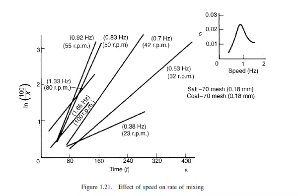
taken round by centrifugal action. If fine particles are put in at the bottom and coarse on the top, then no mixing occurs on rotation and the coarse material remains on top. If the coarse particles are put at the bottom and the fine on top, then on rotation mixing occurs to an appreciable extent, although on further rotation Y falls, and the coarse particles settle out on the top. This is shown in Figure 1.22 which shows a maximum degree of mixing. Again, with particles of the same size but differing density, the denser migrate to the bottom and the lighter to the top. Thus, if the lighter particles are put in at the bottom and the heavier at the top, rotation of the drum will give improved mixing to a given value, after which the heavier particles will settle to the bottom. This kind of analysis of simple mixers has been made by BLUMBERG and MARITZ(23) and by KRAMERS(21), although the results of their experiments are little more than qualitative. BROTHMAN et al.(24) have given an alternative theory for the process of mixing of solid particles, which has been described as a shuffling process. It is proposed that, as mixing takes place, there will be an increasing chance that a sample of a given size intercepts more than one part of the interface, and hence the number of mixed samples will increase
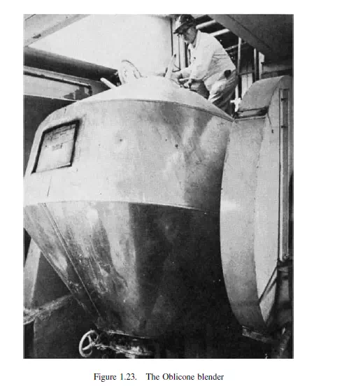
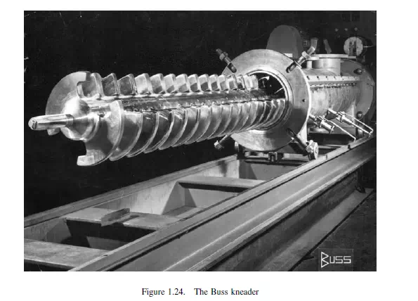
less rapidly than the surface. This is further described by HERDAN(2). The application of some of these ideas to continuous mixing has been attempted by ANCKWERTS(25,26). Two different types of industrial mixers are illustrated in Figures 1.23 and 1.24. The Oblicone blender, which is available in sizes from 0.3 to 3 m, is used where ease of cleaning and 100 per cent discharge is essential, such as in the pharmaceutical, food or metal powder industries. The Buss kneader shown in Figure 1.24 is a continuous mixing or kneading machine in which the characteristic feature is that a reciprocating motion is superimposed on the rotation of the kneading screw, resulting in the interaction of specially profiled screw flights with rows of kneading teeth in the casing. The motion of the screw causes the kneading teeth to pass between the flights of the screw at each stroke backwards and forwards. In this manner, a positive exchange of material occurs both in axial and radial directions, resulting in a homogeneous distribution of all components in a short casing length and with a short residence time.