Three major factors play an important role in determining insulation type and thickness. Here, we’ll focus on resolving the thickness issue since many manufacturing facilities have a “standard” type of insulation that they use. The three key factors to examine are:
1. Economics
2. Safety
3. Process Conditions
Each situation must be studied to determine how to meet each one of these criteria. First, we’ll examine each aspect individually, then we’ll see how to consider all three for an example.
Economics
Economic thickness of insulation is a well documented calculation procedure. The calculations typically take in the entire scope of the installation including plant depreciation to wind speed. Data charts for calculating the economic thickness of insulation are widely available.
Example of Economic Thickness Calculation
Using the tables above, assuming a 6.0 in pipe at 500 °F in an indoor setting with an energy cost of $5.00/million Btu, what is the economic thickness?
Answer: Finding the corresponding block to 6.0 in pipe and $5.00/million Btu energy costs, we see temperatures of 250 °F, 600 °F, 650 °F, and 850 °F. Since our temperature does not meet 600 °F, we use the thickness before it. In this case, 250 °F or 1 1/2 inches of insulation. At 600 °F, we would increase to 2.0 inches of insulation.
Economic thickness charts from other sources will work in much the same way as this example.
Safety
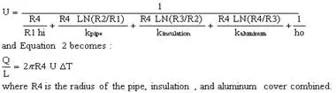
Pipes that are readily accessible by workers are subject to safety constraints. The recommended safe “touch” temperature range is from 130 °F to 150 °F (54.4 °C to 65.5 °C). Insulation calculations should aim to keep the outside temperature of the insulation around 140 °F (60 °C). An additional tool employed to help meet this goal is aluminum covering wrapped around the outside of the insulation. Aluminum’s thermal conductivity of 209 W/m K does not offer much resistance to heat transfer, but it does act as another resistance while also holding the insulation in place. Typical thickness of aluminum used for this purpose ranges from 0.2 mm to 0.4 mm. The addition of aluminum adds another resistance term to Equation 1 when calculating the total heat loss:
 | Eq. (3) |
However, when considering safety, engineers need a quick way to calculate the surface temperature that will come into contact with the workers. This can be done with equations or the use of charts. We start by looking at another diagram:
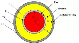
At steady state, the heat transfer rate will be the same for each layer:
 | Eq. (4) |
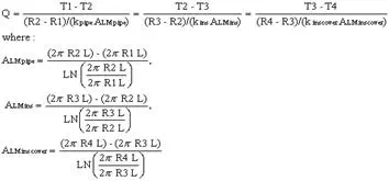
Rearranging Equation 4 by solving the three expressions for the temperature difference yields:
| Eq. (5) |
Each term in the denominator of Equation 5 is referred to as the “resistance” of each layer. We will define this as Rs and rewrite the equation as:
| Eq. (6) |
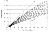 |
| Figure 4: Equivalent ThicknessChart for Calcium Silicate Insulation |
Since the heat loss is constant for each layer, use Equation 4 to calculate Q from the bare pipe, then solve Equation 6 for T4 (surface temperature). Use the economic thickness of your insulation as a basis for your calculation, after all, if the most affordable layer of insulation is safe, that’s the one you’d want to use. If the economic thickness results in too high a surface temperature, repeat the calculation by increasing the insulation thickness by 1/2 inch each time until a safe touch temperature is reached.
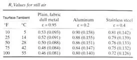
As you can see, using heat balance equations is certainly a valid means of estimating surface temperatures, but it may not always be the fastest. Charts are available that utilize a characteristic called “equivalent thickness” to simplify the heat balance equations. This correlation also uses the surface resistance of the outer covering of the pipe. Figure 4 shows the equivalent thickness chart for calcium silicate insulation. Table 5 shows surface resistances for three popular covering materials for insulation.
 |
With the help of Figure 4 and Table 5 (or similar data for another material you may be dealing with), the relation:
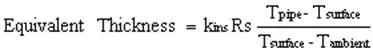 | Eq. (7) |
can be used to easily determine how much insulation will be needed to achieve a specific surface temperature. Let’s look at an example to illustrate the various uses of this equation.
Example of Outer Surface Temperature Determination
Your supervisor asks you to install insulation on a new pipe in the plant. Recently, two workers suffered severe burns while incidentally touching the new piping so safety is of primary concern. He instructs you to be sure that this incident does not repeat itself. The pipe contains a heat transfer fluid at 850 °F (454 °C). The ambient temperature is usually near 85 °F (29.4 °C). After checking the supplies that you have available, you notice that you have calcium silicate insulation and aluminum available for covering. You would like to insulate the 16 inch pipe for a surface temperature of 130 °F.
Tsurface – Tambient = 130 °F – 85 °F = 45 °F, from Table 5 we estimate a Rs value for aluminum at 0.865 h ft2 °F/Btu.
Taverage = (850 °F + 85 °F)/2 = 467.5 °F (242 °C), from Figure 1 we estimate a thermal conductivity of 0.0365 Btu/h ft °F (0.06317 W/m °C) for calcium silicate insulation.

Equivalent Thickness = 6.1 in (155 mm)
From Figure 4 above, an equivalent thickness of 6 in corresponds to an actual thickness of nearly 5.0 in of insulation.
Insulation Process Conditions
The temperature of a fluid inside an insulated pipe is an important process variable that must be considered in many situations. Consider the length of pipe connecting two pieces of process equipment shown below:
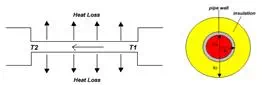
In order to predict T2 for a given insulation thickness, we first make the following assumptions:
1. Constant fluid heat capacity over the fluid temperature range
2. Constant ambient temperature
3. Constant thermal conductivity for fluid, pipe, and insulation
4. Constant overall heat transfer coefficient
5. Turbulent flow inside pipe
6. 15 mph wind for outdoor calculations
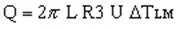
where
 | Eq. (8) |
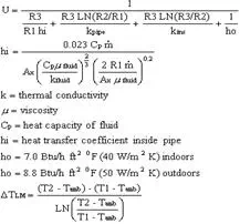
and another heat balance equation yields:
 | Eq. (9) |
Setting Equation 8 equal to Equation 9 and solving for T2 yields:
| Eq. (10) |
Equation 10 provides another useful tool for analyzing insulation and its impact on a process. Equation 10 has been incorporated into the “Insulated Pipe Temperature Prediction Spreadsheet” available in the Download Section.
One example may be the importance of designing insulation thickness to prevent condensation on cold lines. Usually, when we hear the word “insulation” we instantly think of hot lines. However, there are times when insulation is used to prevent heat from entering a line. In this situation, the dew point temperature of the ambient air must be considered. Table 6 and Table 7 show dewpoint temperatures as a function of relative humidity and dry bulb temperatures.
| Table 6: Dew PointTemperatures of Air(Fahrenheit) | ||
  |
It is crucial that sufficient insulation is added so that the outer temperature of the insulation remains abovethe dewpoint temperature. At the dewpoint temperature, moisture in the air will condense onto the insulation and essentially ruin it.
Special Case
For the case of a bare pipe running outside, the chart below can be used to adjust the external heat transfer coefficient from 50 W/m2 K (8.8 Btu/h ft2 °F) to account for temperature difference and wind velocity:
 |
| Figure 6: Bare Pipe External HeatTransfer Coefficient Adjustment |
Practical Example

In the figure above, a typical reactor feed preheater (interchanger) is shown. The heat exchanger resides on the first level of the structure while the reactor is on the second level. During construction, stream 2 was not insulated because it runs from the exchanger directly to the ceiling away from workers so it posed no safety risk. The reaction is endothermic, so heat is supplied by a Dowtherm jacket surrounding the vessel. The equivalent length of the pipe containing stream 2 is 100 meters. A recent rise is fuel oil costs (which is used to heat the Dowtherm) has prompted the company to search for ways to conserve energy. With the data provided below, you recognize an opportunity for energy savings. Any increase in the reactor feed temperature will reduce the reactor duty and save money. What is the current reactor entrance temperature compared with the entrance temperature after applying the economic insulation thickness to the pipe?
Data:
Calcium silicate insulation
Temperature of stream 2 exiting the heat exchanger is 400 °C (752 °F)
Ambient temperature is 23.8 °C (75 °F)
Mass flow = 350,000 kg/h (771,470 lbs/h)
Rinside pipe = R1 = 101.6 mm (4.0 in)
Routside pipe = R2 = 108.0 mm (4.25 in)
Thermal conductivity of pipe = kpipe = 30 W/m K (56.2 Btu/h ft °F)
Ambient air heat transfer coefficient = ho = 50 W/m2 K (8.8 Btu/h ft2 °F)
Fluid heat capacity = Cpfluid = 2.57 kJ/kg K (2.0 Btu/lb °F)
Fluid thermal conductivity = kfluid = 0.60 W/m K (1.12 Btu/h ft °F)
Fluid viscosity = ufluid = 5.2 cP
Energy costs = $4.74/million kJ ($5.00/million Btu)
Equivalent length of pipe = 100 meters (328 feet)
Calculations:
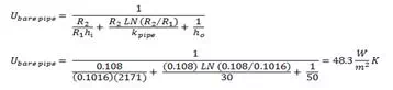
First, we’ll assume little or no wind affects the pipe heat loss and we’ll estimate the heat loss from the bare pipe:
Now, we’ll estimate the radiant heat 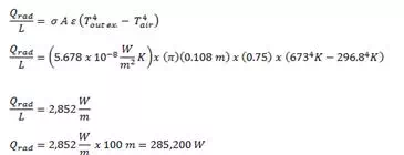 losses:
where: σ = Stefan-Boltzmann constant = 5.678 x 10⁻⁸ W/m2 K
A = circumference of pipe to the outer diameter, m
ε = emissivity of pipe material, taken at 673 K, assume 0.75
T = absolute temperatures, K
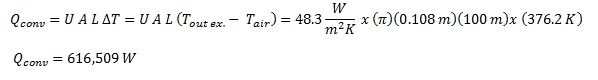
Now, we’ll estimate the losses due to convection:
and we’ll add these together to arrive at the total heat loss for the bare pipe:

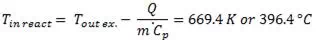
We can now calculate the temperature entering the reactor from the heat exchanger for the bare pipe scenario:
Now, we perform a similar analysis for the insulated pipe:
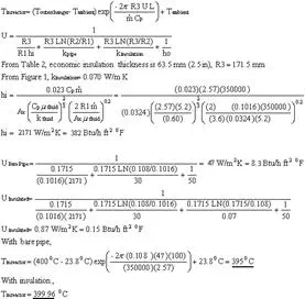
Temperature difference with insulation is 3.56 0C. While this doesn’t sound too dramatic, consider the energy savings over one year with the insulation:
Q = mass flow x Cpfluid x temperature difference
Q = (350,000 kg/h)(2.57 kJ/kg K)(3.56 K) = 3,202,220 kJ/h
3,202,220 kJ/h x 8760 hours/year = 28,051 million kJ/year
28,051 million kJ/year x $4.74/million kJ = $132,961 per year
By insulating the pipe, energy costs have decreased by nearly $133,000 per year
Summary
There are many factors to consider when thinking about insulation. Insulation save money for certain, but it can also be effective as a safety and process control device. Insulation can be used to regulate process temperatures, protect workers from serious injury, and save thousands of dollars in energy costs. One should never overlook it’s usefulness. It’s also bad practice to consider only one of the important factors discussed in this article. The key is to consider all factors that will be affected by installing insulation on a pipe or any other piece of equipment.